Predicting CLV (demo Python)
Customer Lifetime Value prediction
The problem
In this notebook we look at the data we got via this Kaggle dataset (CreditCard_dataset). It involves the car insurance customer lifetime value.
Customer Lifetime Value Prediction( CLV ) value refers to net profit attributed to the entire future relationship with a customer. A bank will use different predictive analytic approaches to predict the revenue that can be generated from any customer in the future. This helps the banks in segmentating the customers in specific groups based on their CLV.
Identifying customers with high future values will enable the organization to keep maintaining good relationships with such customers. It can be done by investing more time and resources on them such as better prices, offers, discounts, customer care services, etc.
Finding and engaging reliable and profitable customers has always been a great challenge for banks. With the increasing competition, the banks need to keep a check on each and every activity of their customers for utilizing their resources effectively.
To solve this problem, Data Science in banking is being used for extracting actionable insights concerning customer behaviors and expectations. Using Data Science models for predicting the CLV of a customer will help a bank to take some suitable decisions for their growth and profit.

Import the important libraries / packages
These packages are needed to load and use the dataset
In [1]:
import pandas as pd #we use this to load, read and transform the dataset
import numpy as np #we use this for statistical analysis
import matplotlib.pyplot as plt #we use this to visualize the dataset
import seaborn as sns #we use this to make countplots
import sklearn.metrics as sklm #This is to test the models
Load and explore the dataset
The data is all in one csv file. In this next step I will first load the data to see how this looks like
In [2]:
#here we load the data
data = pd.read_csv('/kaggle/input/credit-card-data/Fn-UseC_-Marketing-Customer-Value-Analysis.csv')
#and immediately I would like to see how this dataset looks like
data.head()
Out[2]:
| Customer | State | Customer Lifetime Value | Response | Coverage | Education | Effective To Date | EmploymentStatus | Gender | Income | … | Months Since Policy Inception | Number of Open Complaints | Number of Policies | Policy Type | Policy | Renew Offer Type | Sales Channel | Total Claim Amount | Vehicle Class | Vehicle Size | |
|---|---|---|---|---|---|---|---|---|---|---|---|---|---|---|---|---|---|---|---|---|---|
| 0 | BU79786 | Washington | 2763.519279 | No | Basic | Bachelor | 2/24/11 | Employed | F | 56274 | … | 5 | 0 | 1 | Corporate Auto | Corporate L3 | Offer1 | Agent | 384.811147 | Two-Door Car | Medsize |
| 1 | QZ44356 | Arizona | 6979.535903 | No | Extended | Bachelor | 1/31/11 | Unemployed | F | 0 | … | 42 | 0 | 8 | Personal Auto | Personal L3 | Offer3 | Agent | 1131.464935 | Four-Door Car | Medsize |
| 2 | AI49188 | Nevada | 12887.431650 | No | Premium | Bachelor | 2/19/11 | Employed | F | 48767 | … | 38 | 0 | 2 | Personal Auto | Personal L3 | Offer1 | Agent | 566.472247 | Two-Door Car | Medsize |
| 3 | WW63253 | California | 7645.861827 | No | Basic | Bachelor | 1/20/11 | Unemployed | M | 0 | … | 65 | 0 | 7 | Corporate Auto | Corporate L2 | Offer1 | Call Center | 529.881344 | SUV | Medsize |
| 4 | HB64268 | Washington | 2813.692575 | No | Basic | Bachelor | 2/3/11 | Employed | M | 43836 | … | 44 | 0 | 1 | Personal Auto | Personal L1 | Offer1 | Agent | 138.130879 | Four-Door Car | Medsize |
5 rows × 24 columns
In [3]:
#now let’s look closer at the dataset we got

It seems that we have a lot of text / category information (these are of the Dtype ‘object’) and a few numerical columns (Dtypes ‘int64’ and ‘float64’).
The column ‘Customer Lifetime Value’ is the column we would like to predict.
In [4]:
Out[4]:
(9134, 24)
The dataset consists of 9134 rows and 24 columns.
In [5]:
Out[5]:
| Customer Lifetime Value | Income | Monthly Premium Auto | Months Since Last Claim | Months Since Policy Inception | Number of Open Complaints | Number of Policies | Total Claim Amount | |
|---|---|---|---|---|---|---|---|---|
| count | 9134.000000 | 9134.000000 | 9134.000000 | 9134.000000 | 9134.000000 | 9134.000000 | 9134.000000 | 9134.000000 |
| mean | 8004.940475 | 37657.380009 | 93.219291 | 15.097000 | 48.064594 | 0.384388 | 2.966170 | 434.088794 |
| std | 6870.967608 | 30379.904734 | 34.407967 | 10.073257 | 27.905991 | 0.910384 | 2.390182 | 290.500092 |
| min | 1898.007675 | 0.000000 | 61.000000 | 0.000000 | 0.000000 | 0.000000 | 1.000000 | 0.099007 |
| 25% | 3994.251794 | 0.000000 | 68.000000 | 6.000000 | 24.000000 | 0.000000 | 1.000000 | 272.258244 |
| 50% | 5780.182197 | 33889.500000 | 83.000000 | 14.000000 | 48.000000 | 0.000000 | 2.000000 | 383.945434 |
| 75% | 8962.167041 | 62320.000000 | 109.000000 | 23.000000 | 71.000000 | 0.000000 | 4.000000 | 547.514839 |
| max | 83325.381190 | 99981.000000 | 298.000000 | 35.000000 | 99.000000 | 5.000000 | 9.000000 | 2893.239678 |
It seems that we have some strange outliers for the CLV and claim amounts. We will look and handle these later on.
In [6]:
Out[6]:
| Customer | State | Response | Coverage | Education | Effective To Date | EmploymentStatus | Gender | Location Code | Marital Status | Policy Type | Policy | Renew Offer Type | Sales Channel | Vehicle Class | Vehicle Size | |
|---|---|---|---|---|---|---|---|---|---|---|---|---|---|---|---|---|
| count | 9134 | 9134 | 9134 | 9134 | 9134 | 9134 | 9134 | 9134 | 9134 | 9134 | 9134 | 9134 | 9134 | 9134 | 9134 | 9134 |
| unique | 9134 | 5 | 2 | 3 | 5 | 59 | 5 | 2 | 3 | 3 | 3 | 9 | 4 | 4 | 6 | 3 |
| top | YD27780 | California | No | Basic | Bachelor | 1/10/11 | Employed | F | Suburban | Married | Personal Auto | Personal L3 | Offer1 | Agent | Four-Door Car | Medsize |
| freq | 1 | 3150 | 7826 | 5568 | 2748 | 195 | 5698 | 4658 | 5779 | 5298 | 6788 | 3426 | 3752 | 3477 | 4621 | 6424 |
In [7]:
#Let's see what the options are in the text columns with two or three options (the objects)
print('Response: '+ str(data['Response'].unique()))
print('Coverage: '+ str(data['Coverage'].unique()))
print('Education: '+ str(data['Education'].unique()))
print('Employment Status: '+ str(data['EmploymentStatus'].unique()))
print('Gender: ' + str(data['Gender'].unique()))
print('Location Code: ' + str(data['Location Code'].unique()))
print('Married: ' + str(data['Marital Status'].unique()))
print('Policy Type: ' + str(data['Policy Type'].unique()))
print('Vehicle Size: ' + str(data['Vehicle Size'].unique()))

Customer Lifetime Value
As Customer Lifetime Value is the column we want to predict, let’s explore this column in the training dataset.
The formula to calculate the CLV:
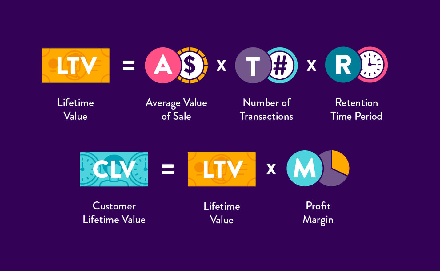
In [8]:
#As this is a numeric, thus continous number, I will use a scatterplot to see if there is a pattern.
plt.hist(data['Customer Lifetime Value'], bins = 10)
plt.title("Customer Lifetime Value") #Assign title
plt.xlabel("Value") #Assign x label
plt.ylabel("Customers") #Assign y label
plt.show()

In [9]:
plt.boxplot(data[‘Customer Lifetime Value’])
Out[9]:


In [10]:
#We see that there are some great outliers here.
#let’s look closer to these outliers over 50000
outliers = data[data[‘Customer Lifetime Value’] > 50000]
Out[10]:
| Customer | State | Customer Lifetime Value | Response | Coverage | Education | Effective To Date | EmploymentStatus | Gender | Income | … | Months Since Policy Inception | Number of Open Complaints | Number of Policies | Policy Type | Policy | Renew Offer Type | Sales Channel | Total Claim Amount | Vehicle Class | Vehicle Size | |
|---|---|---|---|---|---|---|---|---|---|---|---|---|---|---|---|---|---|---|---|---|---|
| 79 | OM82309 | California | 58166.55351 | No | Basic | Bachelor | 2/27/11 | Employed | M | 61321 | … | 30 | 1 | 2 | Personal Auto | Personal L3 | Offer2 | Branch | 427.631210 | Luxury Car | Small |
| 1974 | YC54142 | Washington | 74228.51604 | No | Extended | High School or Below | 1/26/11 | Unemployed | M | 0 | … | 34 | 0 | 2 | Personal Auto | Personal L1 | Offer1 | Branch | 1742.400000 | Luxury Car | Medsize |
| 2190 | KI58952 | California | 51337.90677 | No | Premium | College | 2/24/11 | Employed | F | 72794 | … | 47 | 1 | 2 | Personal Auto | Personal L2 | Offer1 | Web | 50.454459 | SUV | Large |
| 2908 | EN65835 | Arizona | 58753.88046 | No | Premium | Bachelor | 1/6/11 | Employed | F | 24964 | … | 84 | 0 | 2 | Personal Auto | Personal L2 | Offer2 | Agent | 888.000000 | SUV | Medsize |
| 3145 | CL79250 | Nevada | 52811.49112 | No | Basic | Bachelor | 1/8/11 | Unemployed | M | 0 | … | 70 | 0 | 2 | Corporate Auto | Corporate L2 | Offer2 | Agent | 873.600000 | Luxury Car | Small |
| 3760 | AZ84403 | Oregon | 61850.18803 | No | Extended | College | 2/4/11 | Unemployed | F | 0 | … | 29 | 0 | 2 | Personal Auto | Personal L1 | Offer3 | Branch | 1142.400000 | Luxury SUV | Medsize |
| 4126 | JT47995 | Arizona | 60556.19213 | No | Extended | College | 1/1/11 | Unemployed | F | 0 | … | 45 | 0 | 2 | Personal Auto | Personal L3 | Offer1 | Web | 979.200000 | Luxury SUV | Large |
| 4915 | DU50092 | Oregon | 56675.93768 | No | Premium | College | 1/24/11 | Employed | F | 77237 | … | 93 | 0 | 2 | Personal Auto | Personal L1 | Offer4 | Web | 1358.400000 | Luxury SUV | Medsize |
| 5279 | SK66747 | Washington | 66025.75407 | No | Basic | Bachelor | 2/22/11 | Employed | M | 33481 | … | 46 | 0 | 2 | Personal Auto | Personal L3 | Offer1 | Agent | 1194.892002 | Luxury SUV | Medsize |
| 5716 | FQ61281 | Oregon | 83325.38119 | No | Extended | High School or Below | 1/31/11 | Employed | M | 58958 | … | 74 | 0 | 2 | Personal Auto | Personal L3 | Offer1 | Call Center | 1108.800000 | Luxury Car | Small |
| 6252 | BP23267 | California | 73225.95652 | No | Extended | Bachelor | 2/9/11 | Employed | F | 39547 | … | 21 | 0 | 2 | Personal Auto | Personal L3 | Offer1 | Branch | 969.600000 | Luxury SUV | Medsize |
| 6461 | OY68395 | Oregon | 55277.44589 | No | Basic | High School or Below | 1/30/11 | Employed | F | 40740 | … | 60 | 0 | 2 | Personal Auto | Personal L2 | Offer1 | Web | 950.400000 | Luxury SUV | Large |
| 6554 | AH58807 | Arizona | 51426.24815 | No | Basic | College | 1/9/11 | Employed | F | 84650 | … | 39 | 3 | 2 | Personal Auto | Personal L2 | Offer1 | Agent | 660.474274 | Luxury Car | Medsize |
| 6569 | LW64678 | California | 51016.06704 | No | Premium | Master | 2/19/11 | Employed | F | 25167 | … | 76 | 0 | 2 | Personal Auto | Personal L3 | Offer2 | Agent | 422.494292 | SUV | Small |
| 6584 | XF89906 | Arizona | 58207.12842 | No | Extended | High School or Below | 1/13/11 | Disabled | M | 29295 | … | 50 | 0 | 2 | Personal Auto | Personal L3 | Offer1 | Agent | 1328.839129 | Luxury SUV | Large |
| 7283 | KH55886 | Oregon | 67907.27050 | No | Premium | Bachelor | 2/5/11 | Employed | M | 78310 | … | 18 | 1 | 2 | Personal Auto | Personal L1 | Offer1 | Agent | 151.711475 | Sports Car | Medsize |
| 7303 | FB95288 | California | 64618.75715 | No | Extended | High School or Below | 1/17/11 | Unemployed | M | 0 | … | 40 | 1 | 2 | Personal Auto | Personal L3 | Offer1 | Branch | 1562.400000 | Luxury Car | Small |
| 7556 | JZ23377 | Oregon | 57520.50151 | No | Premium | College | 1/20/11 | Employed | F | 48367 | … | 34 | 0 | 2 | Personal Auto | Personal L3 | Offer2 | Branch | 772.800000 | SUV | Medsize |
| 7835 | QT84069 | Oregon | 50568.25912 | No | Extended | Master | 2/28/11 | Employed | M | 82081 | … | 62 | 0 | 2 | Personal Auto | Personal L1 | Offer2 | Branch | 753.760098 | Luxury SUV | Small |
| 8825 | US30122 | California | 61134.68307 | No | Basic | College | 2/28/11 | Unemployed | M | 0 | … | 75 | 0 | 2 | Corporate Auto | Corporate L3 | Offer2 | Branch | 2275.265075 | Luxury Car | Medsize |
20 rows × 24 columns
In [11]:

Looks like there are only 20 rows of the 9134 rows that have a lifetime value of more than 50000. We will leave this as is for now
Handling missing values
Let’s continue with handling the missing values in this dataset. Let’s see where and how many missing values there are in this dataset.
In [12]:
#let’s look in what columns there are missing values
data.isnull().sum().sort_values(ascending = False)
Out[12]:

There seem to be no missing values in this dataset.
Making the text columns Numeric
We first need to make all column input numeric to use them further on. This is what I will do now.
In [13]:
#First we drop the customer column, as this is a unique identifier and will bias the model
data = data.drop(labels = [‘Customer’], axis = 1)
In [14]:
#let’s load the required packages
from sklearn.preprocessing import LabelEncoder
In [15]:
# Let's transform the categorical variables to continous variables
column_names = ['Response', 'Coverage', 'Education', 'Effective To Date', 'EmploymentStatus',
'Gender', 'Location Code', 'Marital Status',
'Policy Type', 'Policy', 'Renew Offer Type',
'Sales Channel', 'Vehicle Class', 'Vehicle Size', 'State']
for col in column_names:
     data[col] = le.fit_transform(data[col])
data.head()
Out[15]:
| State | Customer Lifetime Value | Response | Coverage | Education | Effective To Date | EmploymentStatus | Gender | Income | Location Code | … | Months Since Policy Inception | Number of Open Complaints | Number of Policies | Policy Type | Policy | Renew Offer Type | Sales Channel | Total Claim Amount | Vehicle Class | Vehicle Size | |
|---|---|---|---|---|---|---|---|---|---|---|---|---|---|---|---|---|---|---|---|---|---|
| 0 | 4 | 2763.519279 | 0 | 0 | 0 | 47 | 1 | 0 | 56274 | 1 | … | 5 | 0 | 1 | 0 | 2 | 0 | 0 | 384.811147 | 5 | 1 |
| 1 | 0 | 6979.535903 | 0 | 1 | 0 | 24 | 4 | 0 | 0 | 1 | … | 42 | 0 | 8 | 1 | 5 | 2 | 0 | 1131.464935 | 0 | 1 |
| 2 | 2 | 12887.431650 | 0 | 2 | 0 | 41 | 1 | 0 | 48767 | 1 | … | 38 | 0 | 2 | 1 | 5 | 0 | 0 | 566.472247 | 5 | 1 |
| 3 | 1 | 7645.861827 | 0 | 0 | 0 | 12 | 4 | 1 | 0 | 1 | … | 65 | 0 | 7 | 0 | 1 | 0 | 2 | 529.881344 | 3 | 1 |
| 4 | 4 | 2813.692575 | 0 | 0 | 0 | 52 | 1 | 1 | 43836 | 0 | … | 44 | 0 | 1 | 1 | 3 | 0 | 0 | 138.130879 | 0 | 1 |
5 rows × 23 columns
In [16]:
Out[16]:

As my model can not handle floats, we will change these to integers.
In [17]:
data['Customer Lifetime Value'] = data['Customer Lifetime Value'].astype(int)
data['Total Claim Amount'] = data['Total Claim Amount'].astype(int)
Most important features
Let’s continue by looking at the most important features according to two different tests. Than we will use the top ones to train and test our first model.
In [18]:
#First we need to split the dataset in the y-column (the target) and the components (X), the independent columns.
#This is needed as we need to use the X columns to predict the y in the model.
y = data['Customer Lifetime Value'] #the column we want to predict
X = data.drop(labels = ['Customer Lifetime Value'], axis = 1) #independent columns
In [19]:
from sklearn.feature_selection import SelectKBest
from sklearn.feature_selection import chi2
#apply SelectKBest class to extract top 10 best features
bestfeatures = SelectKBest(score_func=chi2, k='all')
fit = bestfeatures.fit(X,y)
dfscores = pd.DataFrame(fit.scores_)
dfcolumns = pd.DataFrame(X.columns)
#concat two dataframes for better visualization
featureScores = pd.concat([dfcolumns,dfscores],axis=1)
featureScores.columns = ['Name of the column','Score'] #naming the dataframe columns
print(featureScores.nlargest(10,'Score')) #print 10 best features

In [20]:
#get correlations of each features in dataset
corrmat = data.corr()
top_corr_features = corrmat.index
plt.figure(figsize=(20,10))
#plot heat map
g=sns.heatmap(data[top_corr_features].corr(),annot=True,cmap="RdYlGn")

What pop’s out when looking at the correlations for the CLV is the column ‘Monthly Premium Auto’ and the ‘Total Claim Amount’ These might be the best features to use.
Seems that the feature selection models differ a bit in which feature is the most important. For the first test I will keep:
- Total Claim Amount (high in all both tests)
- Monthly Premium Auto (high in all both tests and the highest in the correlation)
- Income (high in two tests)
- Months Since Policy Inception (High in the best features test)
- Coverage (High in the correlation)
Machine learning Model
We want to predict a continous number, therefore we need a linear regression model.
In [21]:
from sklearn.linear_model import LinearRegression
Split the dataset in train and test
Before we are going to use the model choosen, we will first split the dataset in a train and test set. This because we want to test the performance of the model on the training set and to be able to check it’s accuracy.
In [22]:
from sklearn.model_selection import train_test_split
#First try with the 5 most important features
X_5 = data[['Total Claim Amount', 'Monthly Premium Auto', 'Income', 'Coverage', 'Months Since Policy Inception']] #independent columns chosen
y = data['Customer Lifetime Value'] #target column
#I want to withhold 30 % of the trainset to perform the tests
X_train, X_test, y_train, y_test= train_test_split(X_5,y, test_size=0.3 , random_state = 25)
In [23]:
print('Shape of X_train is: ', X_train.shape)
print('Shape of X_test is: ', X_test.shape)
print('Shape of Y_train is: ', y_train.shape)
print('Shape of y_test is: ', y_test.shape)

In [24]:
#To check the model, I want to build a check:
import math
def print_metrics(y_true, y_predicted, n_parameters):
## First compute R^2 and the adjusted R^2
r2 = sklm.r2_score(y_true, y_predicted)
r2_adj = r2 - (n_parameters - 1)/(y_true.shape[0] - n_parameters) * (1 - r2)
## Print the usual metrics and the R^2 values
print('Mean Square Error = ' + str(sklm.mean_squared_error(y_true, y_predicted)))
print('Root Mean Square Error = ' + str(math.sqrt(sklm.mean_squared_error(y_true, y_predicted))))
print('Mean Absolute Error = ' + str(sklm.mean_absolute_error(y_true, y_predicted)))
print('Median Absolute Error = ' + str(sklm.median_absolute_error(y_true, y_predicted)))
print('R^2 = ' + str(r2))
print('Adjusted R^2 = ' + str(r2_adj))
Linear Regression on 5 features
Let’s try the model
In [25]:
# Linear regression model
Out[25]:
LinearRegression()
In [26]:
Predictions = model_5.predict(X_test)
print_metrics(y_test, Predictions, 5)

Hmmm, that is not a good result, just over 14% reliable…
Linear Regression on all
Let’s try the model on all features to see if this improves
In [27]:
#I want to withhold 30 % of the trainset to perform the tests
X_train, X_test, y_train, y_test= train_test_split(X,y, test_size=0.3 , random_state = 25)
print('Shape of X_train is: ', X_train.shape)
print('Shape of X_test is: ', X_test.shape)
print('Shape of Y_train is: ', y_train.shape)
print('Shape of y_test is: ', y_test.shape)

In [28]:
# Linear regression model
Out[28]:
LinearRegression()
In [29]:
Predictions = model.predict(X_test)
print_metrics(y_test, Predictions, 22)

This is even worse.
Conclusion
This model does not perform well to predict the CLV, as the CLV data is highly skewed. To improve the prediction, we could try to normalize the distribution of the CLV column. I will try this here below using Box Cox and Log (two different methods)
In [30]:
#to see the CLV data as is (without having the extremes removed)
data.hist(‘Customer Lifetime Value’, bins = 10)

In [31]:
#Chech the skewness, if p < 0.05 it is skewed
clv = data[‘Customer Lifetime Value’]
from scipy.stats import shapiro
/opt/conda/lib/python3.7/site-packages/scipy/stats/morestats.py:1676: UserWarning: p-value may not be accurate for N > 5000.
warnings.warn(“p-value may not be accurate for N > 5000.”)
Out[31]:
0.0
In [32]:
#as this does not work, let’s continue with the log function
Out[32]:
<matplotlib.axes._subplots.AxesSubplot at 0x7ff0ec64ca90>

In [33]:
print('Shape of X_train is: ', X_train.shape)
print('Shape of X_test is: ', X_test.shape)
print('Shape of Y_train is: ', y_train.shape)
print('Shape of y_test is: ', y_test.shape)
Out[33]:
<matplotlib.axes._subplots.AxesSubplot at 0x7ff0ec597ed0>

BoxCox improved the normal distribution a bit better. Let’s try our linear regression now.
In [34]:
#I want to withhold 30 % of the trainset to perform the tests
X_train, X_test, y_train, y_test= train_test_split(X_5,boxcox_clv, test_size=0.3 , random_state = 25)
In [35]:
model_5.fit(X_train, y_train)
Out[35]:
LinearRegression()
In [36]:
Predictions_box = model_5.predict(X_test)
print_metrics(y_test, Predictions_box, 5)

We can see a slight improvement to 18,5% now. But we need to do further feature improvement to better the result.
Source: https://www.kaggle.com/renatevankempen/predicting-clv